
Adapted From: Introductory Statistics: Concepts, Models, and Applications
David W. Stockburger
Comments in italics are from Linda Woolf
CORRELATION
The Pearson Product-Moment Correlation Coefficient (r), or correlation coefficient for short is a measure of the degree of linear relationship between two variables, usually labeled X and Y. While in regression the emphasis is on predicting one variable from the other, in correlation the emphasis is on the degree to which a linear model may describe the relationship between two variables. In regression the interest is directional, one variable is predicted and the other is the predictor; in correlation the interest is non-directional, the relationship is the critical aspect.
The correlation coefficient may take on any value between plus and minus one.

The sign of the correlation coefficient (+ , -) defines the direction of the relationship, either positive or negative. A positive correlation coefficient means that as the value of one variable increases, the value of the other variable increases; as one decreases the other decreases. A negative correlation coefficient indicates that as one variable increases, the other decreases, and vice-versa.
Remember that correlation does not mean causation. One can not draw cause and effect conclusions based on correlation. There are two reasons why we can not make causal statements:
Taking the absolute value of the correlation coefficient measures the strength of the relationship. A correlation coefficient of r=.50 indicates a stronger degree of linear relationship than one of r=.40. Likewise a correlation coefficient of r=-.50 shows a greater degree of relationship than one of r=.40. Thus a correlation coefficient of zero (r=0.0) indicates the absence of a linear relationship and correlation coefficients of r=+1.0 and r=-1.0 indicate a perfect linear relationship.
The correlation coefficient may be understood by various means, each of which will now be examined in turn.
To evaluate the degree of relationship, one looks at both the slope of the line that would best fit through the data points as well as the degree of scatter from that same line. In correlation, we do not draw the line; in linear regression, we compute the position of the line. The more dispersed the data points, the lower the correlation. The closer all of the data points are to the line, in other words the less scatter, the higher the degree of correlation.
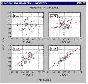
The scatterplots presented below perhaps best illustrate how the correlation coefficient changes as the linear relationship between the two variables is altered. When r=0.0 the points scatter widely about the plot, the majority falling roughly in the shape of a circle. As the linear relationship increases, the circle becomes more and more elliptical in shape until the limiting case is reached (r=1.00 or r=-1.00) and all the points fall on a straight line.
A number of scatterplots and their associated correlation coefficients are presented below in order that the student may better estimate the value of the correlation coefficient based on a scatterplot in the associated computer exercise.
When examining the scatterplots below, examine both the size (degree of the relationship) as well as sign (positive or negative correlation).
r = 1.00
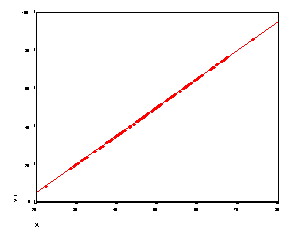
r = -.54
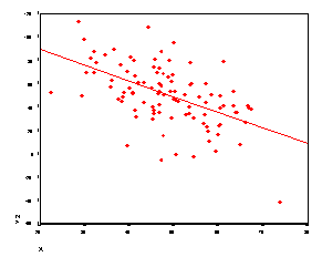
r = .85

r = -.94

r = .42
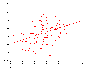
r = -.33
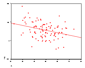
r = .17
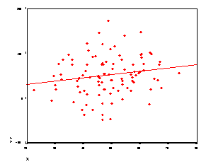
r = .39
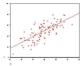
More examples
The correlation coefficient is the slope (b) of the regression line when both the X and Y variables have been converted to z-scores. The larger the size of the correlation coefficient, the steeper the slope. This is related to the difference between the intuitive regression line and the actual regression line discussed above.
This interpretation of the correlation coefficient is perhaps best illustrated with an example involving numbers. The raw score values of the X and Y variables are presented in the first two columns of the following table. The second two columns are the X and Y columns transformed using the z-score transformation.
That is, the mean is subtracted from each raw score in the X and Y columns and then the result is divided by the sample standard deviation. The table appears as follows:
|
X |
Y |
zX |
zY |
|
|
12 |
33 |
-1.07 |
-0.61 |
|
|
15 |
31 |
-0.07 |
-1.38 |
|
|
19 |
35 |
-0.20 |
0.15 |
|
|
25 |
37 |
0.55 |
.92 |
|
|
32 |
37 |
1.42 |
.92 |
|
|
20.60 |
34.60 |
0.0 |
0.0 |
|
|
|
8.02 |
2.61 |
1.0 |
1.0 |
There are two points to be made with the above numbers: (1) the correlation coefficient is invariant under a linear transformation of either X and/or Y, and (2) the slope of the regression line when both X and Y have been transformed to z-scores is the correlation coefficient.
Computing the correlation coefficient first with the raw scores X and Y yields r=0.85. Next computing the correlation coefficient with zX and zY yields the same value, r=0.85. Since the z-score transformation is a special case of a linear transformation (X' = a + bX), it may be proven that the correlation coefficient is invariant (doesn't change) under a linear transformation of either X and/or Y. The reader may verify this by computing the correlation coefficient using X and zY or Y and zX. What this means essentially is that changing the scale of either the X or the Y variable will not change the size of the correlation coefficient, as long as the transformation conforms to the requirements of a linear transformation.
The squared correlation coefficient (r2) is the proportion of variance in Y that can be accounted for by knowing X. Conversely, it is the proportion of variance in X that can be accounted for by knowing Y.
The squared correlation coefficient is also known as the coefficient of determination. It is one of the best means for evaluating the strength of a relationship. For example, we know that the correlation between height and weight is approximately r=.70 If we square this number to find the coefficient of determination - r-squared=.49 Thus, 49 percent of one's weight is directly accounted for one's height and vice versa.